Exploring Time Series Feature Extraction Tools in Python using SKTime

Introduction:
In this project we will dive into the realm of feature extraction tools and particularly time series feature extraction tools.
We will be exploring four powerful feature extraction tools for time series data from SKTime library, train each of them on a dataset, explore their capabilities and have a close look on how each of them transforms time series data.
our four candidates for the project:
In this project we will not talk about the accuracy of the models and the algorithms to depth, rather we will focus on the capabilities of the tools and the way each of them transforms the data.
The Feature Extraction Tools:
A quick overview:
SFA takes a time series, breaks it into smaller pieces, analyzes the frequency patterns in each piece using Discrete Fourier Transform (DFT), simplifies those patterns into categories using MFC, and then forms words from these categories.
These words are a condensed representation of the original data, making it easier to analyze and extract meaningful insights.ROCKET generates random convolutional kernels, including random length and dilation. It transforms the time series with two features per kernel. The first feature is global max pooling and the second is proportion of positive values
Essentially,ROCKET takes your time series data and breaks it down into small windows.
For each window, it identifies the highest point (global max) and calculates the proportion of positive values (ppv).
By doing this for many different windows with random sizes and placements, ROCKET can capture various patterns and characteristics of the time series data.
In simpler terms, ROCKET is like a detective scanning through your data with different-sized magnifying glasses, looking for peaks and positive trends. These features help ROCKET understand the underlying patterns in the data better.
Signature Transform maps time series data into a signature space, capturing the sequential order of observations by considering the iterated integrals of the time series.
shortly it utilizes a feature extraction technique based on the theory of iterated integrals.
Random Shapelet Transform offers an efficient alternative to the traditional Shapelet Transform. Firstly, it randomly selects a subset of subsequences from the time series data as potential shapelets, reducing computational complexity. Next, these randomly chosen shapelets are compared to all possible subsequences in the data using a distance metric like Euclidean distance. Finally, features are extracted based on the similarity between each time series and the selected shapelets, providing a concise representation for downstream tasks such as classification.
Requirements:
List of necessary software and tools required to replicate the project.
Python
PIP
Jupyter Lab
Jupyter notebook
General setup:
First we will open a directory for the project.
We will open the directory in the terminal and enter:
jupyter lab
Last We will Create a new jupyter notebook
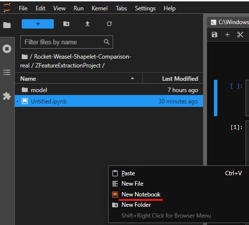
From now on, each below python code block will be written in a separate cell in the notebook.
We will be using:
Sktime library, which provides a unified framework for time series machine learning in Python, to access the dataset and the feature extractions tools.
Joblib for saving and loading the model after it has been fitted on the data.
os - for working with paths, helps save the models relative to the path you are on.
pandas - for converting the time series data we want to transform to a format the algorithms can handle (pandas.DataFrame).
numba - compiler for Python that translates Python code into optimized machine code, typically targeting the CPU. Will make training process faster.
# Installing the library for the dataset and tools
%pip install sktime
# For saving and loading the fitted (trained) models
%pip install joblib
# A requirement for the algorithms to run
%pip install numba
# For working with paths
import os
import joblib
# For converting data to a format the transform function knows how to handle
import pandas as pd
Data Preparation:
The dataset we will be using is the UCR UEA time series classification archive and we are going to access it from sktime library using the load_UCR_UEA_dataset() function.
Currently, sktime provides access to 63 datasets of the UCR UEA dataset which offers a comprehensive collection of labeled time series datasets for research and benchmarking purposes.
# Import sktime function for loading a specific UCR UEA dataset
from sktime.datasets import load_UCR_UEA_dataset
For this project we will be using the InlineSkate dataset from the UCR UEA archive.
We will extract the training data as x_train and y_train, x_train will contain a list of equally sized segments, each segment contains measurements, and y_train will contain the labels of the segments.
The size of x_train and y_train must be equal because every segment has a corresponding label.
We will use this data for fitting the transformers on the time series data, and we will use the first two segments of the x_train data for showing how each feature extraction tool transforms the time series data
# Extract the training data of the InlineSkate DB, We will use the same train data for all 4 feature extractions tools
x_train, y_train = load_UCR_UEA_dataset("InlineSkate", split="train", return_X_y=True)
Lets look on how many segments and labels x_train and y_train contains
# Prnt the num of segments
print(len(x_train)) # Output is 100
# Prnt the num of labels
print(len(y_train)) # Output is 100
And on x_train itself
# A little insight into the x train data
x_train
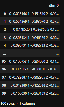
- We can see that we have 100 rows which means we have 100 segment of data.
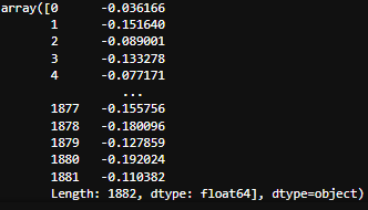
Now lets take a look on the measurements inside the first and the second segments.
# Lets take a look on the first segment
single_time_series = x_train.values[0]
single_time_series
# Lets take a look on the second segment
single_time_series1 = x_train.values[1]
single_time_series1
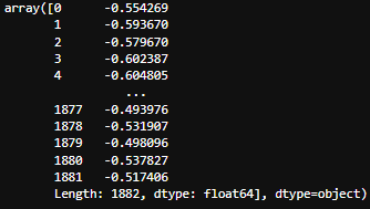
- we can see that each window contains 1882 float values.
So to conclude we have 1882 * 100 = 188,200 total measurements inside the x_train data.
For using the transform() function of each feature extraction tool on the first and the second segments will need to convert the data to pandas.DataFrame
# Getting the first segment ready for transformation using a trained transformer
single_time_series_df = pd.DataFrame({"first_window": single_time_series})
# Getting the second window ready for transformation using a trained transformer
single_time_series_df1 = pd.DataFrame({"second_window": single_time_series1})
Now all the data is ready for experimentation with the tools.
Experimentation
In this section we will use the x_train data for fitting each transformer, and the transform() function of each fitted transformer to exhibit how each tool extracts its features from the time series data.
We will create a new directory (in the same hierarchy as the jupyter notebook) called "model" and a function for saving the fitted transformers inside said directory.
def save_model(transformer_name, fitted_model):
    """
    Save a fitted model to a specified directory.

    Parameters:
    transformer_name (str): Name of the transformer or model.
    fitted_model: Fitted model object to be saved.

    Returns:
    None

    Example:
    save_model("SFA", sfa_fitted_transformmer)
    """
    # Specify the directory and filename where you want to save the model
    save_directory = './model/'
    model_filename = f"{transformer_name}-InlineSkate.pkl"

    # Combine the directory and filename to create the full file path
    full_model_path = os.path.join(save_directory, model_filename)

    # Save the trained model to the specified directory
    joblib.dump(fitted_model, full_model_path)
SFA
First we will import the transformer from sktime.
# Import the time series tranformer - SFA
from sktime.transformations.panel.dictionary_based import SFA
We will fit the SFA transformer on the x_train and y_train data and save the fitted model.
# Initialize SFA transformer
sfa_transformer = SFA()
# Fit data
sfa_transformer.fit(x_train, y_train)
# Save the fitted model
save_model("SFA", sfa_transformer)
After the above code has finished running (1.29 seconds for me), a model named: "SFA-InlineSkate.pkl" should appear in the "model" directory.
For loading the model again in the future you can use:
# Load the model if exists
sfa_transformer = joblib.load("./model/SFA-InlineSkate.pkl")
Now, lets transform the first and the second segments we prepared (single_time_series_df and single_time_series_df1) using the fitted SFA transformer.
# Transform the first segment using fitted SFA transformer
transformed_sfa_window = sfa_transformer.transform(single_time_series_df)
# Transform the second segment using fitted SFA transformer
transformed_sfa_window1 = sfa_transformer.transform(single_time_series_df1)
lets have a look on the transformed data.
As you might remember each segment has 1882 measurements in it so let us examine the features themselves and the count of features within a segment after the transformation.
The first segment:
# Print the number of featuers inside an original segment
print("number of features in a window before transformation:", len(x_train.values[0][0]))
# Print the number of unique featuers (words) inside a transformed first segment
print("number of features (words) in a window after transformation:", len(transformed_sfa_window[0][0]))
# Print the amount of total words inside the transformend first segment
print("The total frequency of all the words inside the trandformed window:", sum(transformed_sfa_window[0][0].values()))
print("------------------------------------------------------------------------------------------------------------------------------------------")
print("The transformed window:")
print(transformed_sfa_window)
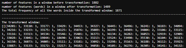
We can see the first segment, which had 1882 floats in it, has been transformed to a dictionary.
A dictionary that contains 1489 unique keys, where the keys are the words(represented as integers) and the values are the frequency of each word in the window (how many times it was captured inside the segment).So, if we sum all the frequencies of the words we get a total of 1871 words captured in the segment.
Thus we can conclude that 1882 - 1871 = 11 fewer distinct features or patterns captured in the symbolic representation compared to the raw measurements.This process allows us to capture important characteristics of the data while reducing its complexity, making it easier to analyze and interpret.
The second segment:
# Print the number of featuers inside an original segment
print("number of features in a window before transformation:", len(x_train.values[0][0]))
# Print the number of unique featuers (words) inside the transformed second segment
print("number of features (words) in a window after transformation:", len(transformed_sfa_window1[0][0]))
# Print the amount of total words inside the transformend second segment
print("The total frequency of all the words inside the trandformed window:", sum(transformed_sfa_window1[0][0].values()))
print("------------------------------------------------------------------------------------------------------------------------------------------")
print("The transformed window:")
print(transformed_sfa_window1)
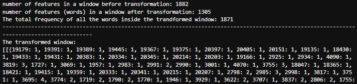
We can see the second segment, which had 1882 floats in it, has been transformed to a dictionary.
A dictionary that contains 1305 unique keys, where the keys are the words(represented as integers) and the values are the frequency of each word in the window (how many times it was captured inside the segment).So, if we sum all the frequencies of the words we get a total of 1871 words captured in the segment.
Thus we can conclude that 1882 - 1871 = 11 fewer distinct features or patterns captured in the symbolic representation compared to the raw measurements.
For the purpose of exhibiting the total number of features and unique features after transformation, we will use the transform() function on all the data (x_train).
# Get x_train data ready for transformation
transformed_sfa_series = sfa_transformer.transform(x_train)
transformed_sfa_series

unique_features = set()
num_of_total_keys_in_series = 0
# Iterate on all the dictionaries in the transformed data
for arr in transformed_sfa_series:
    for dictionary in arr:
        # Sum the length of each dictionary -> will give the total features in the transformed time sseries
        num_of_total_keys_in_series += len(dictionary)
        # Add each key of each dictionary to a set -> will generate a set with all the unique keys
        unique_features.update(dictionary.keys())

print("number of features by suming lenghts of dicts:", num_of_total_keys_in_series) # Output: 142315
print("number of unique features by creating a set with the dictionaries keys:", len(unique_features)) # Output: 14982
- We can see that the total number of features after the transformation, which is equal to the summation of the number of keys in each dictionary, is 142,315, to recall x_train contains 188,200 features so the number of features was reduced by 188,200 - 142,315 = 45885.
And the number of unique features, which is equal to the number of unique keys the transformer generated, is 14,982.
From this we can determine that the words (keys) the SFA generates are not unique between different dictionaries (segments).
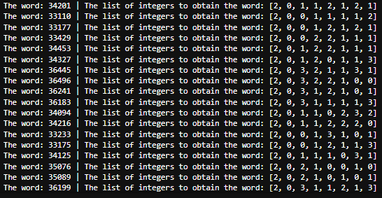
Now let us get a simple overview of the way words (keys) are being created.
For each word (dictionary key) the transformer formed, we can see the set of integers creating the word using the word_list(word) function.
Each window is shortened to an 8 digits word, each digit in a word can be between 0 and 3 [source], for example [2, 0, 1, 1, 2, 1, 2, 1].
So we will use the first segment after the transformation (transformed_sfa_window) in order to show some examples.
#Iterate on all the words (keys) the dictionary representing the first segment contains
for word in transformed_sfa_window[0][0]:
    print(f"The word: {word} | The list of integers to obtain the word: {sfa_transformer.word_list(word)}")
To conclude:
The loading, fitting and saving of the model took 1.29 seconds in total.
The number of features in the first window before transformation is 1882 and after transformation is 1305, leading to a total difference of 393 features which is a decrease in the dimensionality of the feature space.
The amount of measurements inside the first window before the transformation is 1882 and the amount of words detected in the first window after the transformation is 1871 (summing the frequencies of each word inside the first window).
It suggests that there are 11 fewer distinct features or patterns captured in the symbolic representation compared to the raw measurements.The number of features in the second window before transformation is 1882 and after transformation is 1305 (number of unique words), leading to a total difference of 577 features which is a decrease in the dimensionality of the feature space.
The amount of measurements inside the second window before the transformation is 1882 and the amount of words detected in the second window after the transformation is 1871 (summing the frequencies of each word inside the second window).
It suggests that there are 11 fewer distinct features or patterns captured in the symbolic representation compared to the raw measurements.The total number of features across the whole time series data before the transformation is 188,200 and after the transformation is 142,315, leading to a difference of 45,885 features in total.
The algorithm produced a total of 14,982 words, this number reflects the diversity of patterns captured from the time series.
ROCKET
First we will import the transformer from sktime.
# Import the time series tranformer - ROCKET
from sktime.transformations.panel.rocket import Rocket
We will fit the Rocket transformer on the x_train and y_train data and save the fitted model.
# Initialize ROCKET transformer
rocket_transformer = Rocket()
# Fit data
rocket_transformer.fit(x_train, y_train)
# Save the fitted model
save_model("ROCKET", rocket_transformer)
After the above code has finished running (9.01 seconds for me), a model named: "ROCKET-InlineSkate.pkl" should appear in the "model" directory.
For loading the model again in the future you can use:
# Load the model if exists
rocket_transformer = joblib.load("./model/ROCKET-InlineSkate.pkl")
Now, lets transform the first and the second segments we prepared (single_time_series_df and single_time_series_df1) using the fitted ROCKET transformer.
# Transform the first segment using fitted ROCKET transformer
transformed_rocket_window = rocket_transformer.transform(single_time_series_df)
# Transform the seecond segment using fitted ROCKET transformer
transformed_rocket_window1 = rocket_transformer.transform(single_time_series_df1)
Lets have a look on the transformed data.
As you might remember each segment has 1882 measurements in it so let us examine the features themselves and the count of features within a segment after the transformation.
The first segment:
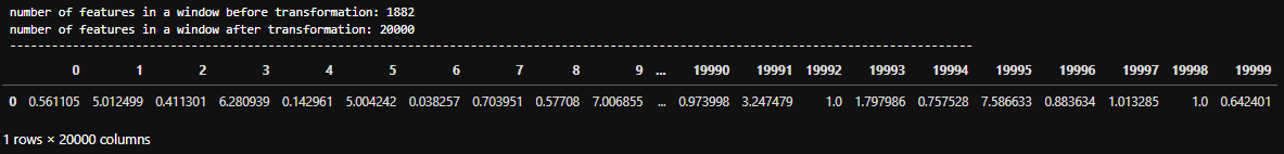
print("number of features in a window before transformation:", len(x_train.values[0][0]))
# Prints the number of features (number of columns) ROCKET algorithm extracted from the time series data
print("number of features in a window after transformation:", transformed_rocket_window.shape[1])
print("------------------------------------------------------------------------------------------------------------------------------------------")
print(type(transformed_rocket_window))
transformed_rocket_window
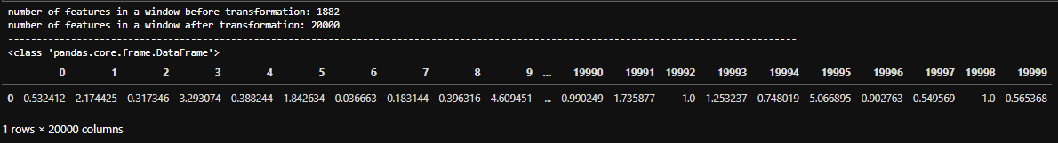
We can see the first segment, which had 1882 floats in it, has been transformed to a pandas.DataFrame with 1 row and 20,000 columns, in terms of dimensions, it's a one-dimensional dataset with 20,000 features or variables.
So the number of features inside the first segment has increased by 20,000 - 1882 = 18,118.
As we can see in the documentation the ROCKET algorithm number of kernels is 10,00 by default and each kernel function generates two features: the first feature is the proportion of positive values (ppv), and the second feature is the global maximum (max) value, so it result in total of 20,000 features per segment.So to conclude, The ROCKET algorithm increases the feature space by transforming the original data into a higher-dimensional representation and the number of features is dependent on the number of kernels.
The Second segment:
# Print the number of featuers inside an original segment
print("number of features in a window before transformation:", len(x_train.values[0][0]))
# Prints the number of features (number of columns) ROCKET algorithm extracted from the time series data
print("number of features in a window after transformation:", transformed_rocket_window1.shape[1])
print("------------------------------------------------------------------------------------------------------------------------------------------")
transformed_rocket_window1
- Just like the first segment, the number of features inside the second segment has increased by 20,000 - 1882 = 18,118 and the total number of features inside the segment is 20,000.
To conclude:
The loading, fitting and saving of the model took 9.01 seconds in total.
The transformation applied by ROCKET is consistent across different segments of the dataset, after a transformation a segment will have 20,000 features.
The number of features in the first window before transformation is 1882 and after transformation is 20,0000, leading to a total difference of 18,118 features which is a increase in the dimensionality of the feature space.
The total number of features across the whole time series data before the transformation is 188,200 and after the transformation is 20,000 * 100 = 2,000,000 (num_of_features in a segment * num_of_segments), leading to a difference of 1,811,800 features in total.
Signature Transform
In order to be able to run, Signature Transform requires python version to be less than 3.10 and installing esig.
First we will install esig using pip
%pip install esig
Second we will import the transformer from sktime.
# Import the time series tranformer - Signature Transform
from sktime.transformations.panel.signature_based._signature_method import SignatureTransformer
We will fit the Shapelet transformer on the x_train and y_train data and save the fitted model.
# Initialize signature transformer
signature_transformer = SignatureTransformer()
# Fit data
signature_transformer .fit(x_train, y_train)
# Save the fitted model
save_model("Signature", signature_transformer)
After the above code has finished running (less than a second for me), a model named: "Signature-InlineSkate.pkl" should appear in the "model" directory.
For loading the model again in the future you can use:
# Load the model if exists
signature_transformer= joblib.load("./model/Signature-InlineSkate.pkl")
Now, lets transform the first and the second segments we prepared (single_time_series_df and single_time_series_df1) using the fitted Signature transformer.
# Transform the first segment using fitted Signature transformer
transformed_signature_window = signature_transformer.transform(single_time_series_df)
# Transform the second segment using fitted Signature transformer
transformed_signature_window1 = signature_transformer.transform(single_time_series_df1)
Lets have a look on the transformed data.
As you might remember each segment has 1882 measurements in it so let us examine the features themselves and the count of features within a segment after the transformation.
The first segment:
print("number of features in a window before transformation:", len(x_train.values[0][0]))
# Prints the number of features (number of columns) Signature Transformer extracted from the time series data
print("number of features in a window after transformation:", transformed_signature_window.shape[1])
print("------------------------------------------------------------------------------------------------------------------------------------------")
transformed_signature_window
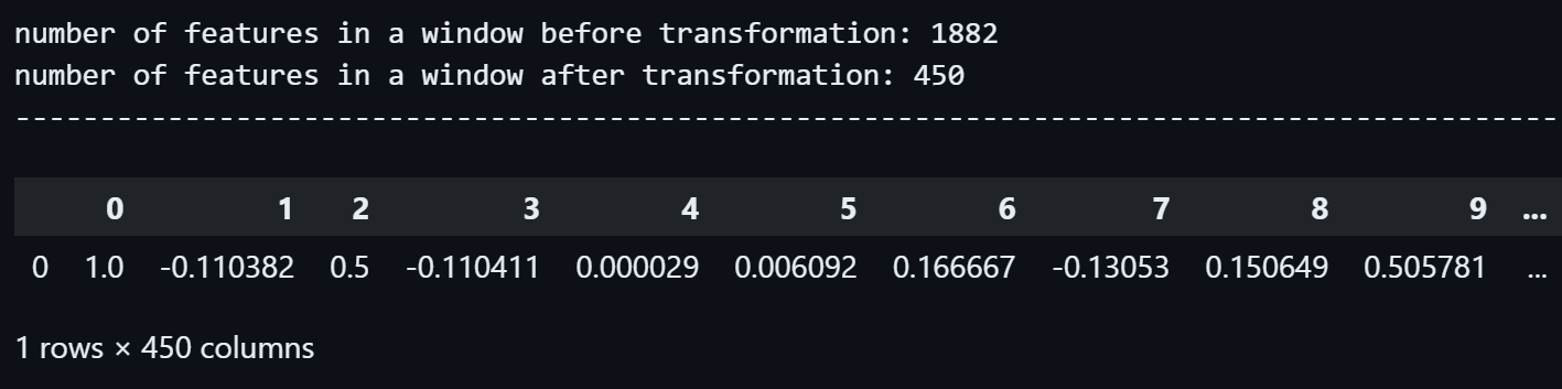
We can see the first segment, which had 1882 floats in it, has been transformed to a pandas.DataFrame with 1 row and 450 columns, in terms of dimensions, it's a one-dimensional dataset with 450 features or variables.
So the number of features inside the first segment has decreased by 1882 - 450 = 1432.
The second segment:
print("number of features in a window before transformation:", len(x_train.values[0][0]))
# Prints the number of features (number of columns) Signature Transformer extracted from the time series data
print("number of features in a window after transformation:", transformed_signature_window1.shape[1])
print("------------------------------------------------------------------------------------------------------------------------------------------")
transformed_signature_window1
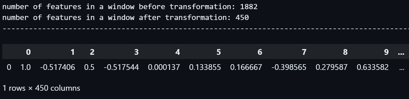
Just like the first segment, we can see that the second segment, which had 1882 floats in it, has been transformed to a pandas.DataFrame with 1 row and 450 columns.
So the number of features inside the second segment has also decreased by 1882 - 450 = 1432.
To conclude:
The loading, fitting and saving of the model took less than one second in total.
The number of features in the first window before transformation is 1882 and after transformation is 450, leading to a total difference of 1432 features which is a decrease in the dimensionality of the feature space.
The fact that the number of features is consistently reduced by the same amount (1432 features) in both windows indicates that the transformation applied by the Signature Transformer is consistent across different segments of the dataset.
The total number of features across the whole time series data before the transformation is 188,200 and after the transformation is 450 * 100 = 45,000 (num_of_features in a segment * num_of_segments), leading to a difference of 143,200 features in total.
Random Shapelet Transform
First we will import the transformer from sktime.
# Import the time series tranformer - Shapelet Transform
from sktime.transformations.panel.shapelet_transform import RandomShapeletTransform
We will fit the Shapelet transformer on the x_train and y_train data and save the fitted model.
# Initialize Shapelet transformer
shapelet _transformer = RandomShapeletTransform()
# Fit data
shapelet_transformer.fit(x_train, y_train)
# Save the fitted model
save_model("RandomShapelet", shapelet _transformer)
After the above code has finished running ( 258.2 seconds for me), a model named: "RandomShapelet-InlineSkate.pkl" should appear in the "model" directory.
For loading the model again in the future you can use:
# Load the model if exists
shapelet_transformer = joblib.load("./model/RandomShapelet-InlineSkate.pkl")
Now, lets transform the first and the second segments we prepared (single_time_series_df and single_time_series_df1) using the fitted Random Shapelet transformer.
# Transform single time series using Random Shapelet transformer
transformed_shapelet_window = shapelet_transformer.transform(single_time_series_df)
# Transform the second window of the time series
transformed_shapelet_window1 = shapelet_transformer.transform(single_time_series_df1)
Lets have a look on the transformed data.
As you might remember each segment has 1882 measurements in it so let us examine the features themselves and the count of features within a segment after the transformation.
The first segment:
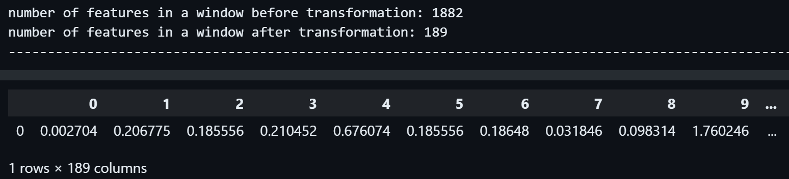
print("number of features in a window before transformation:", len(x_train.values[0][0]))
# Prints the number of features (number of columns) Random Shapelet algorithm extracted from the time series data
print("number of features in a window after transformation:", transformed_shapelet_window.shape[1])
print("------------------------------------------------------------------------------------------------------------------------------------------")
transformed_shapelet_window
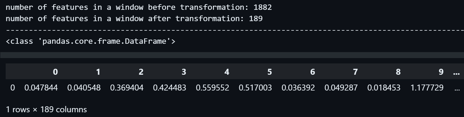
We can see the first segment, which had 1882 floats in it, has been transformed to a pandas.DataFrame with 1 row and 189 columns, in terms of dimensions, it's a one-dimensional dataset with 189 features or variables.
So the number of features inside the first segment has decreased by 1882 - 189 = 1693.
The second segment:
print("number of features in a window before transformation:", len(x_train.values[0][0]))
# Prints the number of features (number of columns) Random Shapelet algorithm algorithm extracted from the time series data
print("number of features in a window after transformation:", transformed_shapelet_window1.shape[1])
print("------------------------------------------------------------------------------------------------------------------------------------------")
transformed_shapelet_window1
Just like the first segment, we can see that the second segment, which had 1882 floats in it, has been transformed to a pandas.DataFrame with 1 row and 189 columns.
So the number of features inside the second segment has also decreased by 1882 - 189 = 1693.
Let us have a glimpse of the shapelets (discriminative subsequences within time series data that capture important patterns) the algorithm as captured from the data.
We will look on the first shapelete.
shapelet_transformer.shapelets[0]
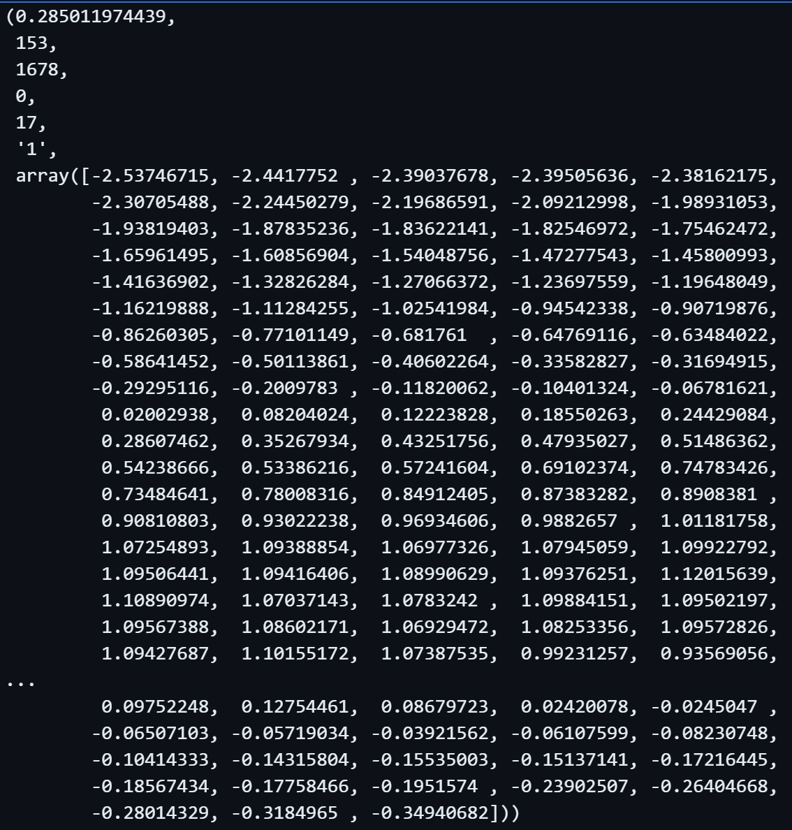
This is the first shapelet extracted from the data.
According to the documentation, each item in the list of shapelets is a tuple containing the following 7 items:
1. shapelet information gain - It measures how well a shapelet can separate different classes within the dataset. In our example the value is 0.2850...2. shapelet length - how many measurments are inside the shapelet. In our example the value is 153.
3. start position the shapelet was extracted from - the start position relative to the segment it was etracted from. In our example the value is 1678 out of 1882 values in a segment.
4. shapelet dimension
5. index of the instance the shapelet was extracted from in fit - The segment number the shapelet was found in. In our example the value is 17 out of the 100 segments.
6. class value of the shapelet - The label of the shapelet. In our example the value is 1.
7. The z-normalised shapelet array - The shapelet itself, which is a part of the timeseries. In our example it's the array.
To conclude:
The loading, fitting and saving of the model took 258.2 seconds in total.
The number of features in the first window before transformation is 1882 and after transformation is 189, leading to a total difference of 1693. features which is a decrease in the dimensionality of the feature space.
The fact that the number of features is consistently reduced by the same amount (1693 features) in both windows indicates that the transformation applied by the Random Shapelet Transformer is consistent across different segments of the dataset.
The total number of features across the whole time series data before the transformation is 188,200 and after the transformation is 189 * 100 = 18,900 (num_of_features in a segment * num_of_segments), leading to a difference of 169,300 features in total.
We can assume that the 189 dominant shapelets we found are used to calculate the distance form them to each other shapelet and than each other shapelet will be classified by the labels of the closest dominant shapelete using a distance function.
Results and Analysis
Let us compare the results we achieved so far.
We will use graphs to exhibit the results.
First, we will import a module that will help us with the graphs.
import matplotlib.pyplot as plt
Second, we will gather the data we achieved from each transformer.
# Data for each transformer
transformers = ['SFA', 'ROCKET', 'Signature Transform', 'Random Shapelet Transform']
time_taken = [1.29, 9.01, 0.2, 258.2]  # Time taken in seconds
num_features_diff = [45885, -1811800, 143200, 169300]  # Difference in number of features after transformation
model_size_kb = [2, 587, 2, 1310]  # Model size in KiloByte
Now we are able to use matplotlib to exhibit the results as graphs.
- Let us take a look on the time each transformer trained on the data.
# Plotting the time taken for each transformer
plt.figure(figsize=(8, 6))
bars = plt.bar(transformers, time_taken, color='skyblue')
plt.xlabel('Transformer')
plt.ylabel('Time Taken (seconds)')
plt.title('Time Taken for Model Loading, Fitting, and Saving')
plt.xticks(rotation=45)  # Rotate x-axis labels
plt.grid(axis='y', linestyle='--', alpha=0.7)

# Adding text labels on top of each bar
for bar, time in zip(bars, time_taken):
    height = bar.get_height()
    plt.text(bar.get_x() + bar.get_width() / 2, height, f'{time:.2f}', ha='center', va='bottom')

plt.tight_layout()
plt.show()
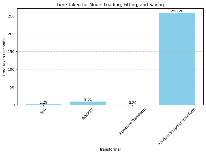
- We can see the Random Shapelet Transformer has taken much more time to "fit" itself in relation to all the other transformers.
- Let us take a look on the space in memory each model takes.
# Plotting the model size for each transformer
plt.figure(figsize=(8, 6))
bars = plt.bar(transformers, model_size_kb, color='lightgreen')
plt.xlabel('Transformer / Model')
plt.ylabel('Model Size (KB)')
plt.title('Model Size in Kilo Bytes')
plt.xticks(rotation=45)  # Rotate x-axis labels
plt.grid(axis='y', linestyle='--', alpha=0.7)

# Adding text labels on top of each bar
for bar, size in zip(bars, model_size_kb):
    height = bar.get_height()
    plt.text(bar.get_x() + bar.get_width() / 2, height, f'{size}', ha='center', va='bottom')

plt.tight_layout()
plt.show()
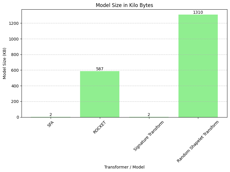
- We can see that SFA and Signature Transform models are of size 2KB which is a very small size, the ROCKET model size is 587KB and the Shapelet model takes the most memory space out of all the models, its size is 1310 KB.
- Let us take a look on the difference in number of features after transformation for each transformer.
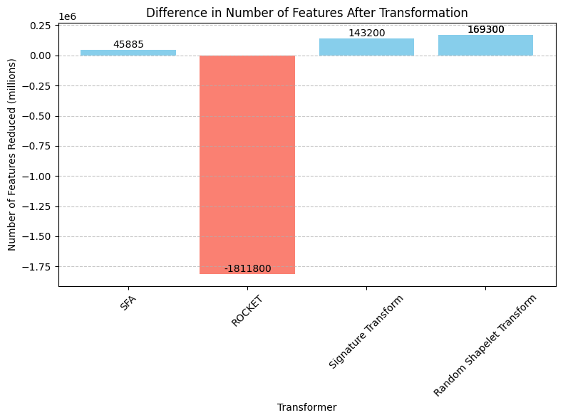
- We can see that the model that has reduced the most features after transformation is Shapelet Transform and that the ROCKET model is the only model that has increased the number of features, and by a lot (1,811,800 features).
In term of ease of use, all algorithms had excellent documentation,but, SFA, ROCKET and Shapelete Transform share the same interface, each should be imported and trained, they are all very easy to use.
In contrast, Signature Transform required python version to be less than 3.10 so I had to download a specific version just to use the algorithm and it required installing esig.
So, to conclude Signature Transform is not hard to use but required more specific requirements in order to be used, thus making it less "easy to use" than the other algorithms.
In terms of the consistency of transformations, particularly regarding the size of the transformed segment, the Signature , ROCKET and Random Shapelet transformers ensure uniformity across different segments of the dataset.
On the other side, SFA does not ensure it, as we saw above, the number of features inside the transformed first and second segments was different.
Int terms of feature insight, the SFA transformer offers an insight to how each word was created, or more specifically, what were the 8 integers that created this word.
And the shapelet transformer offers an insight to the shapelets it extracted from the graph, while The ROCKET and Signature Transform doesn't provide anything special, they can just transform the data.
Future Applications
All the algorithms are pretty much used to the same task which is to extract distinct and unique patterns/features form a time series so in real life applications they can used for analyzing sensor data, finance trends, healthcare data, stocks etc.
As we saw, the Random Shapelet Transformer took the most time to be trained and the size of its model was the highest but it was also the one that reduced the feature space the most.
So, it required the most space and time for training but after the training the feature reduction is the most significant. Thus can be used when there is no time and space limitations.
Rocket was fast, the size of its model was average and it was the only model that increased the amount of features in a segment, but that is also his purpose, ROCKET aims to transform the original time series data into a higher-dimensional representation. This process enables the extraction of meaningful features which in the end makes calculations faster.
SFA and Signature Transform were both super fast, the size of their models was equal and very small (2 KB) making them the most efficient in terms of time and space.
Conclusion:
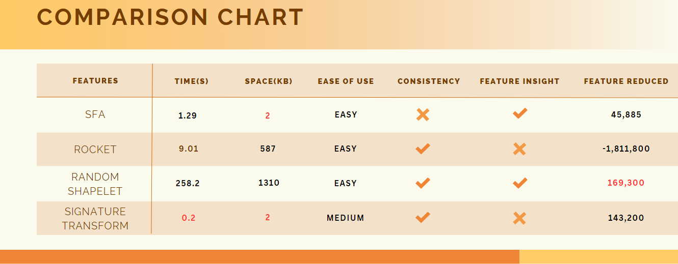
Consistency - Consistency of transformations, particularly regarding the size of the transformed segment.
Feature Reduced - Number of total features reduced after the transformation.
Feature Insight - Does the tool provide deeper feature insight.
This project taught me a lot about time series feature extractions, both theoretically and practically.
From the perspective of the theoretical knowledge I gained, I learned that time series feature extraction is used in a various fields, from analyzing sensors data to financial and medical data and even weather forecasting.
The process mainly involves extracting dominant/distinguishing features from the time series or finding dominant shapes/patterns in the time series data.
From the perspective of the practical knowledge I gained, I learned how to use the sktime library for extracting features form a time series data in various ways, I observed the actual data before and after the transformation to get a better understanding of what each transformer actually does and when it was possible I dived into how and what features were extracted (See SFA and Random Shapelete).
From the perspective of "side knowledge" I gained, I learned how to use matplotlib to exhibit data in graphs, I learned about a lot of libraries that were used in different steps of the project, libraries like pandas, joblib, numba, etc.
References:
Database:
SFA:
[1] Schäfer, Patrick, and Mikael Högqvist. "SFA: a symbolic fourier approximation and index for similarity search in high dimensional datasets." Proceedings of the 15th international conference on extending database technology. 2012,
https://openproceedings.org/2012/conf/edbt/SchaferH12.pdf
ROCKET:
[1] Tan, Chang Wei and Dempster, Angus and Bergmeir, Christoph and Webb, Geoffrey I, "ROCKET: Exceptionally fast and accurate time series classification using random convolutional kernels",2020, https://link.springer.com/article/10.1007/s10618-020-00701-z, https://arxiv.org/abs/1910.13051
Signature Transform:
[1] James Morrill, Adeline Fermanian, Patrick Kidger, Terry Lyons, "A Generalised Signature Method for Multivariate Time Series Feature Extraction",2021,
https://arxiv.org/pdf/2006.00873.pdf
Random Shapelet Transform:
Hills, J., Lines, J., Baranauskas, E. et al. Classification of time series by shapelet transformation. Data Min Knowl Disc**28**, 851–881 (2014). https://doi.org/10.1007/s10618-013-0322-1
[2] A. Bostrom and A. Bagnall, "Binary Shapelet Transform for Multiclass Time Series Classification", Transactions on Large-Scale Data and Knowledge Centered Systems, 32, 2017,
https://link.springer.com/book/10.1007/978-3-662-55696-2
