Introduction
In this project we will dive into the realm of reinforcement learning, we will use two reinforcement learning algorithms, PPO and DQN , for creating AI models capable of playing Mario.
We will train each model 2,000,000 timesteps and will be saving a new model after every 50,000 steps for evaluation purposes, therefore we will have a total of 40 models created by each algorithm.
We will take a deep dive into the algorithms, and for simplicity, instead of comparing and analyzing every model we saved, we will compare the models that were saved after : 50,000 ; 500,000 ; 1,000,000 ; 2,000,000 timesteps.
The Algorithms
Both algorithms were taken from the AI RL library Stable Baselines3.
DQN -Deep Q Network
Challenges addressed by DQN in reinforcement learning:
We don’t have a labeled data set, so how do we know which action is the correct action to perform.
Let’s say we have an agent and it has a task to achieve in the environment, if the environment is a small one and the task is relatively an easy task, we could easily traverse the environment multiple times to build a map of the world which will guide the agent to achieving his target, and create a lookup table which gives you the best option to perform in a certain state the agent is in, This approach is known as Q-learning. But, if the environment is very complicated and there are a lot of actions the agent can perform and every combination of the allowed actions differentiate by the order of the actions the agent took, meaning different actions in different orders will result a different state, than we can’t create an infinite (or finite by way too large) lookup table for each state and the best action to perform.
How DQN handles the challenges:
RL agent learns by trial and error, in our case the data will be generated by having Mario move around the environment and interact with it, every step that Mario takes in the environment generates a 4-tuple called “Experience”
<s, a, s_, r> where:
s is the current state of the agent.
a is the action that he performed.
s_ is the new state as a result of the previous state and the action
r is the reward obtained by performing said action.In DQN, we build our dataset by storing these experiences in a replay Memory (the replay buffer). The replay buffer holds the last N interactions that the agent has with the environment, causing the agent to see this multiple times thus forcing it to learn from its past experiences. So this is basically how the agent can learn from past experience, but how does it label the data.
DQN encodes the information via a state-action value function, also known as Q-values which are a numerical indicator determining how useful it is to perform a certain action in a given state in moving the agent toward its goal. More formally, it is the expected discounted return of performing action ‘a’ in state ‘s’.
We can see by the equation that the Q value of the current state and action depend on the Q value of the next state and action, which will depend on the next state and action and so on.
This recursive property helps us to define the labels to learn on.
DQN handles the first problem by using neural networks to track the vast amount of information.
In DQN, the Q-value is estimated by the neural network, so instead of directly telling which action to perform, the neural network gives us an estimate of the Q-value of each of the possible actions, the agent than selects the action with the highest Q-value.
So the equation above can be updated to:

Now it takes into account the neural network, and after we know the target result and the predicted result the network learns by computing the mean squared error between the target value and the prediction value.

Thus, uses bootstrapping (A technique where an estimate updates another estimate)
It is important to note that this bootstrapping setup lead to some instability issues.
So, we have a network which is updated by computing the error between the predicted-Q and the target-Q but both this values are estimated using the same network, which means after the update, the target-Q value on the very same state will be completely different.
This led to the predicted-Q value and the target-Q value constantly having to play catch up with each other.
To get over this problem, the developers of the algorithm introduced a second network, called the target network.
The target network is an exact copy of the already in use online network with one key difference- the target network never undergoes gradient updates.
Introducing a second network meant that the predicted-Q and target-Q values could now be computed by a separate network, thus keeping the target Q-values relatively constant.
One more key element:
We said earlier that the agent selects the action with the highest Q-value in a certain state, but to be more precise, this is what happens during the testing of the model. In training, we do need the agent to explore the environment, to ensure that he can find a better possible route to the goal, DQN handles this by using epsilon greedy policy, it means that based on a certain criteria, the agent decides whether to act randomly or to perform the action suggested by the network.To summarize:
Data is generated via agent-environment interaction.
Data is stored on the Replay Memory.
Neural Network: Input = State; Output = Q-value per action
Bootstrapping can cause instability => use Target Network, whose sole purpose is to compute the target values.
Deep dive into DQN algorithm
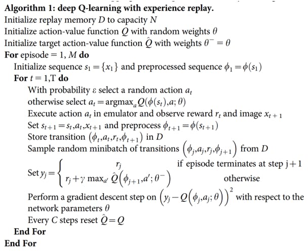
- Mnih, V., Kavukcuoglu, K., Silver, D., et al. (2015). Human-level control through deep reinforcement learning. Nature, 518(7540), 529-533. https://doi.org/10.1038/nature14236
The Replay Memory:
We already established that the Replay Memory is used to store each of the interactions that the agent has with the environment, the Replay Memory is limited to a certain size defined by the user, as the memory fills up all the experiences are removed to make space for the newer ones.
What to do with the samples In the Replay Memory?
We can look at the Replay Memory as an equivalent to the dataset in a supervised learning setting, thus, for the agent to learn from this data, at each iteration we need to feed the neural network mini batches of data which are the samples for it to optimize on, this mini batch is created by randomly sampling from the Replay Memory, the samples are chosen in a random manner because it helps to break correlations in data samples, thus it becomes more sample efficient.
So, the use of the Replay Memory ensures that the agent sees each data point multiple times before the data point is removed from memory.
The Neural Network:
DQN uses Online Network and a Target Network to ensure stability in training, these two are instances of the same network with the update technique being the only difference between them.
The output of the neural network determines how the agent will act, the selected action is the action with the highest Q-value, at least during testing. And during training the algorithm also encourage exploration by an Epsilon-Greedy Policy.
The Epsilon-Greedy Policy works by initializing a threshold value called epsilon, at each step we generate a random number, if the random number is smaller than epsilon than we perform a random action (exploring the environment) otherwise the algorithm will perform the action suggested by the neural network.
Over time, as the model progresses, we would like to rely more on the information we gathered than on random exploration. It is achieved by annealing the epsilon value, so as the agent learns more about the environment, we reduce the epsilon value until it finally reaches a very small number, which will cause the choosing of the random actions (exploration actions) to decrease and relying more on the neural network outputs.
The Q-values:
Numerically indicate how good certain action is in a given state by computing the total discounted reward the agent can expect in the future if it follows the current policy.
Breaking down the algorithm:

- Initialize the replay memory, done by executing s completely random actions for a few timesteps.

- Creating the online network and the target network and set the weights of the target network to be the same as the weights of the online network.

- As part of the training loop, start gathering current observations.
The outer for loop tracks the total number of steps that need to be performed, while the inner for loop tracks the steps in the current episode until terminal state reached.

At each timestep use the epsilon greedy strategy to determine whether to perform a random action or act as the neural network output

Execute the selected action, to obtain the immediate reward and the next state

Store this experience of state, action, reward and next state into the replay memory.

Draw a mini batch of random samples from the memory

Compute the target-Q value using the target network, by accounting for terminal states

Compute the predicted Q-value using the online network and compute the loss between the target and predicted Q’s to update the weights of the online network.

At regular intervals, copy the weights of the online network into the target network.
Summary
DQN is an off-policy algorithm that uses a replay buffer to store past experiences and samples a batch of these experiences to compute the Q-values for each action. It then uses these Q-values to update the action-value function using the Bellman equation. This allows the agent to learn from past experiences and improve its policy over time.
PPO - Proximal Policy Optimization
Challenges addressed by PPO in reinforcement learning:
The training data that is generated, is itself dependent on the current policy because our agent is generating its own training data by interacting with the environment rather than relying on a static data like supervised learning does. This means that the data distribution of our observations and rewards are constantly changing as our agent learns, which is a major cause of instability in the whole training process.
Reinforcement learning also suffers from a very high sensitivity to hyper parameter tuning, in things like initialization for example.
In some cases it is kind of intuitive to understand why this happens, for example if the learning rate is to large we could have a policy update that pushes our policy network into a region of the parameter space where it’s going to collect the next batch of data under a very poor performance policy, causing it to never recover again.
To address many of these problems in the reinforcement learning, the algorithm called PPO was designed by the Open Ai team. The core purpose behind the PPO algorithm was to strike a balance between:
Ease of implementation
Sample efficiency
Ease of tuning
PPO is a policy gradient method, it means that unlike DQN for example, that can learn from stored offline data, PPO learns online means it doesn’t use a replay buffer to store past experiences but instead it learns directly from whatever its agent encounters in the environment and once a batch of experience was used to do a gradient update the experience is than discarded and the policy moves on.
This also means that policy gradient methods are typically less sample efficient than queue learning methods because they only use the collected experience once for doing an update.
Defining the default policy gradient loss:

- Figure 1
πθ - our policy, a neural network that takes the observed states in the environment as an input (sₜ) and suggests actions to take as an output(aₜ)(in our case the states are frames of the game, and the output is the action Mario should take in that frame).
Aₜ - The advantage function that tries to estimate what is the relative value of the selected action in the current state, where the little t represents the current timestep.
In order to compute the reward, we need the discounted sum of rewards and a baseline estimate.
The discounted sum of rewards is a weighted sum of all the rewards the agent got during each timestep in the current episode , the calculation uses a gamma variable ,that goes between 0.9 and 0.99, accounts to the fact that the agent cares more about rewards that its going to get very quickly versus the same reward it would get a 100 timesteps from now.

- Schulman, J., Wolski, F., Dhariwal, P., Radford, A., & Klimov, O. (2017). Proximal Policy Optimization Algorithms. CoRR, abs/1707.06347. http://arxiv.org/abs/1707.06347
The advantage is calculated after the episode sequence was collected form the environment therefore, we already know all the rewards and can calculate the discounted sum of rewards.
The baseline estimate, also called the value function, tries to estimate the discounted sum of rewards from this point onward, so basically, it is trying to guess what the final return is going to be in this episode starting from the current state. During training, the neural network that is representing the value function is going to be frequently updated using the experience that our agent collects from the environment.
So to summarize, we are taking states as an input and the neural network tries to predict what the discounted sum of rewards will be from this state onward, kind of like in supervised learning. The estimate is going to be a noisy estimate because our network is not going to always predict the exact value of that states.
The advantage estimate provided by the advantage function is:
Aₜ = discounted sum of rewards - baseline estimate.
Which will point on how much better was the action that the agent took based on the expectation of what would normally happen in this specific state.
So basically when Aₜ is positive, it means the discounted sum of rewards is better than the baseline estimate, which from the equation above (See Figure 1) will result to a positive outcome, therefore will increase the probability of selecting the actions that the agent took in said trajectory again in the future when the agent encounters the same state.
And when Aₜ is negative it implies that the actions the agent took during the trajectory are worse than the estimated return, which from the equation above (See Figure 1) will result to a negative outcome, resulting decrease of the probability that said actions will be taken again in the future while encountering the same states.
To avoid to large policy updates, which can cause the returned value of the advantage function to be very noisy and lead to destroying your policy until the point it can no longer recover, PPO uses clipping, The main idea is that after an update, the new policy should be not too far from the old policy in order to obtain stable learning that can converge to a good model.
PPO main objective function

- Figure 2
PPO Computes this over a batches of trajectories.
Parameters:
Probability ratio between the new updated policy outputs and the outputs of the previous, old version of the policy network.
Means that the value will be larger than 1 if the actions of the agent are more likely now than it was in the old policy and the value will be between 0 and 1 if the actions are less likely now than it was in the old policy.
- clip(x, a, b)
- clips the value of x between a and b, it returns:
a, if x < a.
b, if x > b.
x otherwise.
The whole purpose of this formula (see Figure 2) is to prevent too big policy updates, if the update is to big it gets clipped to limit the effect of the gradient update.
The effect of the main objective function changes when the advantage (Aₜ) is negative and when it is positive.
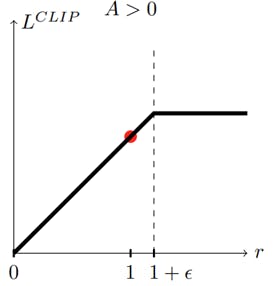
When the advantage is positive (A > 0), means the selected actions of the agent had a better than expected effect on the outcome, when r gets to big (x axis), means that the actions of the agent are much more likely now than it was in the old policy, clip the loss function value, in order to prevent a to big policy update/limit the effect of the gradient update.
Or in a simpler term, if the action was good and it became a lot more probable after the last gradient step don’t keep updating to much or else it might get worse. (Because we know that we have a very noisy advantage function and we don’t want to destroy a policy based on a single estimate).

When the advantage is negative (A < 0), means the selected actions of the agent had a worse than expected effect on the outcome
when r gets closer to 0, means that the actions are less likely now than it was in the old policy, clip the loss function value, prevent doing an update that will hurry to reduce the probability of the selected actions.
When r gets bigger, means that the likelihood of those actions is higher in the current policy than it was in the old policy, than we would like to undo the last gradient step therefore L_clip ends up being negative thus telling us to go the other direction and make the action less probable by an amount proportional to the growth of r (seen by the linear line, when R is bigger than L_clip is smaller). This region in the graph is the only region where the left parameter of the min function is smaller than the right parameter (see Figure 2), thus get returned by the min function, which will cause the reduction in the likelihood of said actions.
So, to summarize, the PPO objective forces the policy updates to be conservative if they move very far away from the current policy, with a very simple objective function that does not require much calculations.
PPO algorithm
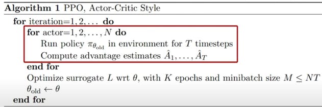
There are two alternating threads in PPO.
In the first one,, the current policy is interacting with the environment, generating episode sequences for which we immediately calculate the advantage function using the fitted baseline estimate for the state values.

And in every so many episodes the second thread is going to collect all this experience and run gradient descent on the policy network using the clipped PPO objective.
And now for the final loss function that is used to train an agent.

Break Down:

- The loss function (see Figure 2) that forces the policy updates to be conservative if they move very far away from the current policy.

- In charge for updating the baseline network based on "how good it is to be in a certain state", or more specifically what is the average amount of discounted rewards that I expect to get from this point onward.

- The entropy term, in charge for making sure that the agent does enough exploration during training.
So in contrast to discrete action policies that output the action choice probabilities, the PPO policy head outputs the parameters of a Gaussian distribution for each available action type, and when running the agent in training mode, the policy will sample from this distributions to get a continuous output value for each action head.
Adding an entropy term will cause the policy to behave a little bit more randomly until the other parts of the objective start dominating, or in other words, the model as started to converge to "a good place".
Summary
PPO is a policy gradient method, the algorithm has a good stability and reliability, is simple to implement and can be used for a wide range of reinforcement learning tasks.
PPO is an on-policy algorithm that directly updates the policy network using the current trajectory of the agent. It uses a trust region optimization method to ensure that the updates to the policy network are conservative and do not deviate too much from the previous policy. This allows the agent to learn more efficiently and stabilize its learning process.
Environment Setup
Project requirements
Python
PIP
Jupyter notebook
gym_super_mario_bros
nes_py.wrappers
PyTorch(in order to use stable_baselines3 algorithms).
tensorboard
tesnorflow
Setup Mario
First we will install gym_super_mario_bros and nes-py, which is an OpenAI Gym environment for Super Mario Bros. & Super Mario Bros. 2 (Lost Levels) on The Nintendo Entertainment System (NES) using the nes-py emulator, which let you play the game with python.
pip install gym_super_mario_bros==7.4.0 nes_py
Than, we will import some modules that will help us in our task:
import gym_super_mario_bros
from nes_py.wrappers import JoypadSpace
from gym_super_mario_bros.actions import SIMPLE_MOVEMENT
Now we will initialize the game:
env = gym_super_mario_bros.make('SuperMarioBros-v0')
Gym is a toolkit for developing and comparing reinforcement learning algorithms.
By default, gym_super_mario_bros environment use actions space of 256 discrete actions which takes a lot of time for an AI model to learn and a lot of space in our computer, at least if we want the AI to make it through the first level.
So, we will use the SIMPLE_MOVEMENT actions list that contains 7 actions: [ [‘NOOP’], [‘right’], [‘right’, A], [‘right’, B], [‘right’, A, B], [A], [‘left’] ] Which will decrease the time it takes for our agent to “learn”.
After that we will wrap our current environment (using nes_py.wrappers) with the JoypadSpace Providing him with the game and the allowed actions to perform.
env = JoypadSpace(env, SIMPLE_MOVEMENT)
The JoypadSpace plays the game with the actions provided to him, It uses a method called: “actions_space.sample()” which chooses a random action from the actions list and performs it in the game.
For our AI to learn, we will use a Reinforcement algorithm which uses a reward as a guideline.
The reward function
The function:
r = v + c + d
The reward is clipped into the range (-15, 15).
The parameters:
v - The difference in agent x values between states
in this case this is instantaneous velocity for the given step
v = x1 - x0
x0 is the x position before the step
x1 is the x position after the step
moving right ⇔ v > 0
moving left ⇔ v < 0
not moving ⇔ v = 0
c - The difference in the game clock between frames
the penalty prevents the agent from standing still
c = c0 - c1
c0 is the clock reading before the step
c1 is the clock reading after the step
no clock tick ⇔ c = 0
clock tick ⇔ c < 0
d - A death penalty that penalizes the agent for dying in a state
this penalty encourages the agent to avoid death
alive ⇔ d = 0
dead ⇔ d = -15
The state
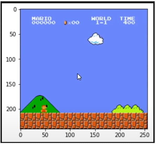
The state is simply one frame of the game, the RGB values represented by matrices of numbers, here is an image representation of an actual state from our program using matplotlib.
For analyzing the actions of our agent in the world later on, we will use the following line of code:
state, reward, done, info = env.step(env.action_space.sample())
To understand what is happening here:
As you might remember, the env variable is the JoypadSpace wrapping the Mario game.
This line of code performs a random step in the game, the variables:
state, reward, done and info hold information about how the random step effected us
State and reward are mentioned and explained above.
The variable “done” is a Boolean indicating if we are alive or not.
And info contains information about the world for example (x and y axis of our agent, collected coins, etc..).
Preprocess The Environment
The focus in this section is how we enabled our model to actually learn and how we improved the learning of our AI by neglecting variables that doesn’t contribute to our learning(insufficient data).
First we will install PyTorch and stable-baselines3, and import other modules that their purpose will be explained later:
!pip install torch==1.10.1+cu113 torchvision==0.11.2+cu113 torchaudio===0.10.1+cu113 -f https://download.pytorch.org/whl/cu113/torch_stable.html
!pip install stable-baselines3[extra]
from gym.wrappers import GrayScaleObservation
from stable_baselines3.common.vec_env import VecFrameStack, DummyVecEnv
Pre-explanation
We need to pre-process our Mario game data before we “AI-fy” it, for this we are going to apply two key pre-processing steps, gray scaling and frame stacking.
Our AI is going to be taking images of the Mario game to learn, a colored image has 3 times as many pixels to process, so converting it to gray scale cuts down the data it has to learn from.
GrayScaleObservation allows us to convert our colored game into a gray scale version, which will cut down the amount of information our AI need to produce.
A colored image is effectively the (height * width * 3 channels), because we need one channel per a color to represent red, green and blue.
If we make it grayscale we actually cut down the amount of data by third.
Frame stacking helps out AI have a context, by stacking consecutive frames we are effectively giving our AI model memory, it will be able to see Mario and his enemies movements.
Vectorization Wrappers:
When implementing our reinforcement learning model we need to vectorize it in order to be able to actually use it with our AI.
We will use stable-baselines3, which is an AI library for reinforcement learning containing different algorithms.
VecFrameStack allows us to work with our stacked environments, it allows us to capture a couple of frames while we are playing Mario, this means that the AI model will be able to see what happened in the last x frames, where x is a number we define, so basically, it will be able to see movements.
Otherwise, let us say we pass just one frame to our AI, it is only going to know what has happened right in this frame, so it doesn’t have any concept of movement or velocity, so we are going to stack frames together in order to train our AI.
DummyVecEnv just wraps out our base environment inside of a vectorization wrapper.
That is basically how we need to transform our model in order to be able to pass it to the AI model.
The environment thus far
This is our current environment
# 1. Create the base environment
env = gym_super_mario_bros.make('SuperMarioBros-v0')
# 2. Simplify the controls
env = JoypadSpace(env, SIMPLE_MOVEMENT)
Using above modules, the improved environment look like this
# 1. Create the base environment
env = gym_super_mario_bros.make('SuperMarioBros-v0')
# 2. Simplify the controls
env = JoypadSpace(env, SIMPLE_MOVEMENT)
# 3. Grayscale
env = GrayScaleObservation(env, keep_dim=True)
# 4. Wrap inside the Dummy Environment
env = DummyVecEnv([lambda: env])
# 5. Stack the frames
env = VecFrameStack(env, 4, channels_order='last')
Train The RL Model
We will train the models using two different reinforcement learning algorithms from stable-baselines3:
PPO - Proximal Policy Optimization
DQN – Deep Q Network.
PPO
First part of the learning process
We will import “os” and BaseCallback to save our models and information about the training.
We will import the PPO algorithm which will be used for the learning process.
# Import os for file path management
import os
# Import PPO for algos
from stable_baselines3 import PPO
# Import Base Callback for saving models
from stable_baselines3.common.callbacks import BaseCallback
We will define a callback which will allow us to save our model every so and so steps, the number of steps will be determined by the value of the argument check_freq and the place where our model will be saved will be determined by the value of the argument save_path.
class TrainAndLoggingCallback(BaseCallback):

    def __init__(self, check_freq, save_path, verbose=1):
        super(TrainAndLoggingCallback, self).__init__(verbose)
        self.check_freq = check_freq
        self.save_path = save_path

    def _init_callback(self):
        if self.save_path is not None:
            os.makedirs(self.save_path, exist_ok=True)

    def _on_step(self):
        if self.n_calls % self.check_freq == 0:
            model_path = os.path.join(self.save_path, 'best_model_{}'.format(self.n_calls))
            self.model.save(model_path)
        return True
We will define two variables that will hold a string representation of the folders' names wherein the model and the log files will be saved.
CHECKPOINT_DIR = './ppo_train/'
LOG_DIR = './ppo_logs/'
We will define the callback variable which will cause the model to be saved automatically every 50,000 steps in the ppo_train folder.
# Setup model saving callback
callback = TrainAndLoggingCallback(check_freq=50000,save_path=CHECKPOINT_DIR)
We will initialize the model providing it the neural network CnnPolicy and the environment.
# This is the AI model started
model = PPO('CnnPolicy', env, verbose=1, tensorboard_log=LOG_DIR, learning_rate=0.000001,n_steps=512)
- CnnPolicy – a neural network that is very fast in processing images (the frames of the game).
And finally, we will start the learning process of the model by telling it to run for 1,000,000 steps.
# Train the AI model, this is where the AI model starts to learn
model.learn(total_timesteps=1000000, callback=callback)
Second part of the learning process
In the second part of the learning, we will load the 1,000,000 model that was saved after the first part of training and let it learn for another 1,000,000 steps and save a model every 50,000 steps in a folder called ppo_train2.
So in total it ran for 2,000,000 steps.
CHECKPOINT_DIR = './ppo_train2/'
callback = TrainAndLoggingCallback(check_freq=50000,save_path=CHECKPOINT_DIR)

# load the model
model = PPO.load(‘./ppo_train/best_model_1000000’)
# env is the environment as seen in the end of the section:"Environment Setup"
model.set_env(env)
model.learn(total_timesteps=1000000, callback=callback)
Side Note:
Those are the default parameters of the PPO algorithm we used:
PPO(policy, env, learning_rate=0.0003, n_steps=2048, batch_size=64, n_epochs=10, gamma=0.99, gae_lambda=0.95, clip_range=0.2, clip_range_vf=None, normalize_advantage=True, ent_coef=0.0, vf_coef=0.5, max_grad_norm=0.5, use_sde=False, sde_sample_freq=-1, target_kl=None, tensorboard_log=None, policy_kwargs=None, verbose=0, seed=None, device='auto', initsetup_model=True).We overridden only below values:
verbose=1
tensorboard_log=LOG_DIR
learning_rate=0.000001
n_steps=512
DQN
First part of the learning process
First, we will import the DQN algorithm.
# Import DQN for algos
from stable_baselines3 import DQN
Then we will run cell that initializes the base environment again.
# 1. Create the base environment
env = gym_super_mario_bros.make('SuperMarioBros-v0')
# 2. Simplify the controls
env = JoypadSpace(env, SIMPLE_MOVEMENT)
# 3. Grayscale
env = GrayScaleObservation(env, keep_dim=True)
# 4. Wrap inside the Dummy Environment
env = DummyVecEnv([lambda: env])
# 5. Stack the frames
env = VecFrameStack(env, 4, channels_order='last')
And define a new folders for the training data and the place where we save the model.
CHECKPOINT_DIR = './dqn_train/'
LOG_DIR = './dqn_logs/'
Then, we will initialize the callback (we defined above) again with the new folders.
callback = TrainAndLoggingCallback(check_freq=50000,save_path=CHECKPOINT_DIR)
And initialize the model with the same neural network and learning rate, but override the default buffer size to be 10,000 instead of 1,000,000 (because of RAM limitations).
model = DQN('CnnPolicy', env, buffer_size=10000, verbose=1, tensorboard_log=LOG_DIR, learning_rate=0.000001)
And finally, we will start the learning process of the model by telling it to run for 1,000,000 steps.
# Train the AI model, this is where the AI model starts to learn
model.learn(total_timesteps=1000000, callback=callback)
Second part of the learning process
In the second part of the learning, we will load the 1,000,000 model that was saved after the first part of training and let it learn for another 1,000,000 steps and save a model every 50,000 steps in a folder called dqn_train2.
So in total it ran for 2,000,000 steps.
CHECKPOINT_DIR = './dqn_train2/'
callback = TrainAndLoggingCallback(check_freq=50000,save_path=CHECKPOINT_DIR)

# load the model
model = DQN.load(‘./dqn_train/best_model_1000000’)
model.set_env(env)
model.learn(total_timesteps=1000000, callback=callback)
Side Note:
Those are the default parameters of the DQN algorithm we used:
DQN(policy, env, learning_rate=0.0001, buffer_size=1000000, learning_starts=50000, batch_size=32, tau=1.0, gamma=0.99, train_freq=4, gradient_steps=1, replay_buffer_class=None, replay_buffer_kwargs=None, optimize_memory_usage=False, target_update_interval=10000, exploration_fraction=0.1, exploration_initial_eps=1.0, exploration_final_eps=0.05, max_grad_norm=10, tensorboard_log=None, policy_kwargs=None, verbose=0, seed=None, device='auto', initsetup_model=True).
We overridden only below values:
buffer_size=10000,
verbose**=**1,
tensorboard_log**=**LOG_DIR,
learning_rate**=**0.000001
Test out The RL Models
So, to summarize what we did in the training process, we let each algorithm (PPO, DQN) run for total of 2,000,000 steps in 2 learning parts, where each part contained 1,000,000 steps, and we saved our model each 50,000 steps, therefore we have a total of 40 models created by each algorithm.
We will load and run those models on the game environment for making a comparison between the real time results each algorithm achieved.
In order to test and run the models, we will make some imports again.
# Import the game
import gym_super_mario_bros
# Import the Joypad wrapper
from nes_py.wrappers import JoypadSpace
# Import the SIMPLIFIED controls
from gym_super_mario_bros.actions import SIMPLE_MOVEMENT
# Import GrayScaling Wrapper
from gym.wrappers import GrayScaleObservation
# Import Vectorization Wrappers
from stable_baselines3.common.vec_env import VecFrameStack, DummyVecEnv
# Import DQN for algos
from stable_baselines3 import DQN
# Import PPO for algos
from stable_baselines3 import PPO
Than we will load the environment the model will be tested on (the game).
# Create the base environment
env = gym_super_mario_bros.make('SuperMarioBros-v0')
# Simplify the controlls
env = JoypadSpace(env, SIMPLE_MOVEMENT)
# Grayscale, we need the keep_dim=True to be able to use are Stack
env = GrayScaleObservation(env, keep_dim=True)
# Wrap inside the dummy environment
env = DummyVecEnv([lambda: env])
# Stack the frames
env = VecFrameStack(env, 4, channels_order='last')
Loading and running the PPO model:
As we mentioned, our PPO models are saved in 2 different directories, each directory had 20 model and was storing the information of 1,000,000 timesteps.
The names of the directories:
ppo_train
ppo_train2
each model is called best_model_x , where x is the number of timesteps in the current run when the model was saved.
In order to load the PPO model we will use the following line of code:
# Load model
model = PPO.load('./ppo_train2/best_model_1000000')
Using this line of code, we will load the 1,000,000 timesteps model of the second part of the training(ppo_train2), which means the 2,000,000 timesteps model.
And in order to run the model and test it we will ran the following lines of code :
# Start the game
state = env.reset()
# Loop through the game
while True:
# Predict the action that the agent should do in the current state        # based on the model
    action, _ = model.predict(state)
    # make the action the model predicted in the game
    state, reward, done, info = env.step(action)
    env.render()
Loading and running the DQN model:
As we mentioned, our DQN models are saved in 2 different directories, each directory had 20 model and was storing the information of 1,000,000 timesteps.
The names of the directories:
dqn_train
dqn_train2
each model is called best_model_x , where x is the number of timesteps in the current run when the model was saved.
In order to load the DQN model we will use the following line of code:
# Load model
model = DQN.load('./dqn_train2/best_model_1000000')
Using this line of code, we will load the 1,000,000 timesteps model of the second part of the training(dqn_train2), which means the 2,000,000 timesteps model.
In order to run the model and test it we will use the following lines of code :
obs = env.reset()
# Loop through the game
while True:
# Predict the action that the agent should do in the current state        # based on the model
    action, _states = model.predict(obs, deterministic=False)
    # make the action the model predicted in the game
    obs, reward, done, info = env.step(action)
    env.render()
    # If Mario died after the last action reset the game
    if done:
      obs = env.reset()
Evaluation of The Models
PPO vs. DQN: Comparison
| PPO | DQN | Implications | |
| Type of algorithm | On-policy | Off-policy | PPO is more sample efficient because it uses the current policy to generate data for the update. DQN is off-policy algorithm that uses a replay buffer to store and reuse past experiences. |
| Sample efficiency | High | Medium | PPO can achieve better performance with less data, DQN requires more data to achieve similar performance. ( PPO uses the current policy to generate data for the update, which makes it more sample efficient. DQN uses a replay buffer to store and reuse past experiences, which requires more data to achieve similar performance) |
| Robustness to hyperparameters | High | Medium | PPO is less sensitive to the choice of hyperparameters, which makes it easier to train and tune. DQN may require more fine-tuning of the hyperparameters. (PPO uses a trust region optimization method which controls the step size) |
| Handling high-dimensional action spaces | Good | Not recommended | PPO can handle high-dimensional action spaces more effectively than DQN, which makes it suitable for a wide range of tasks. DQN is not recommended for tasks with high-dimensional action spaces. |
| Suitable for complex dynamics | Yes | No | PPO is known to have good performance in tasks that have complex dynamics, which makes it a great choice for many real-world applications. DQN is not suitable for tasks with complex dynamics. |
| Suitable for real-world applications | Yes | Yes | PPO is a good choice for real-world applications with complex dynamics and high-dimensional action spaces. DQN is good for tasks without those characteristics and it's more suitable for Atari games. |
| Trust region optimization | Yes | No | PPO uses a trust region optimization method which controls the step size of the update, allowing for more stable and robust training. DQN does not use this method. |
| Learning rate sensitivity | Low | Medium |
The Learning Graphs
In order to see the graphs from the log files each algorithm saved during the training, first use pip to install tensorboard and tesnorflow.
Second, in the cmd go to the path of the log files and run the following command:
tensorboard --logdir=.
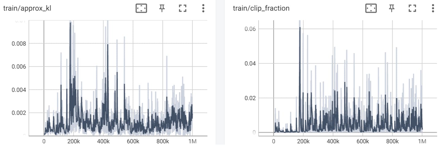
PPO iteration 1 (0 – 1,000,000 timesteps)
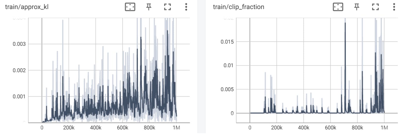

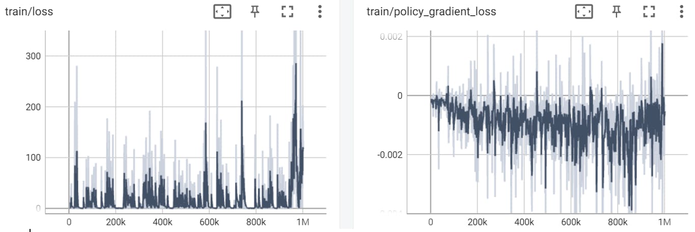
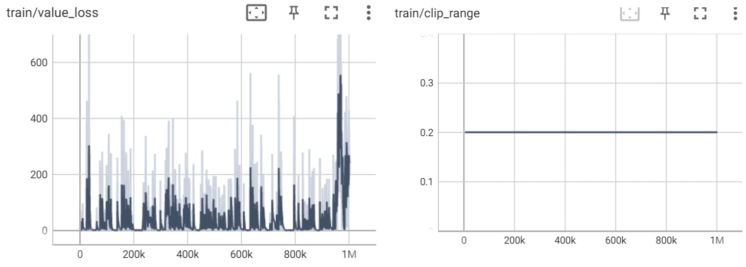
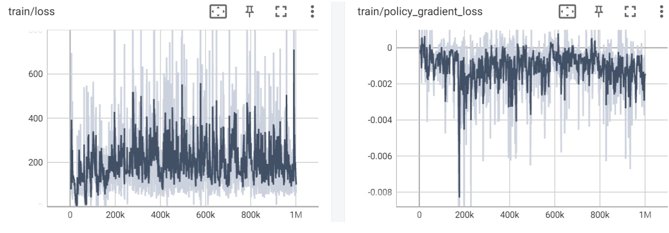
PPO iteration 2 (1,000,000 – 2,000,000 timesteps):


DQN iteration 1 (0 – 1,000,000 timesteps)


DQN iteration 2 (1,000,000 – 2,000,000 timesteps):


Analyzing The Graphs
PPO
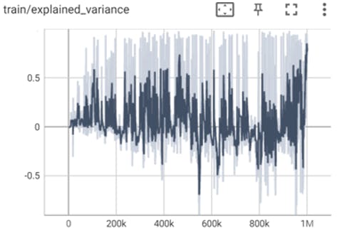
The explained_variance graph after 1,000,000 timesteps:
The explained_variance graph after 2,000,000 timesteps:
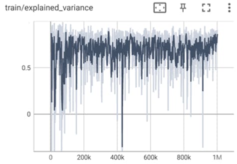
The explained_variance parameter represents the explained variance of the value function.
It measures the degree to which the value function is able to predict the expected returns.
In the first graph we can see that the explained variance is very unstable, means that the model doesn’t make such a good prediction of expected returns, as the learning process continues, in the second graph we can see that the explained variance went up and become more stable, means that the model improved it’s ability to predict the expected returns, thus indicates that the learning process is going well (The model learns).
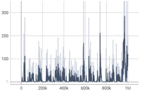
The loss graph after 1,000,000 timesteps:
The loss graph after 2,000,000 timesteps:

This parameter represents the overall loss of the model, which is a combination of the policy gradient loss, value loss, and entropy loss.
We can see in both graphs that the loss value doesn’t decrease over time and actually it increases over time which can suggest on a poor learning or a need in change of the hyper-parameters.
Even above statements, we severe it’s ok and only natural for an agent that is learning from trial and error and that is always expected to encounter new states (whenever it reaches to a point in the game he has never seen before) to make mistakes when it tries to predict the best action to take in these states.
DQN
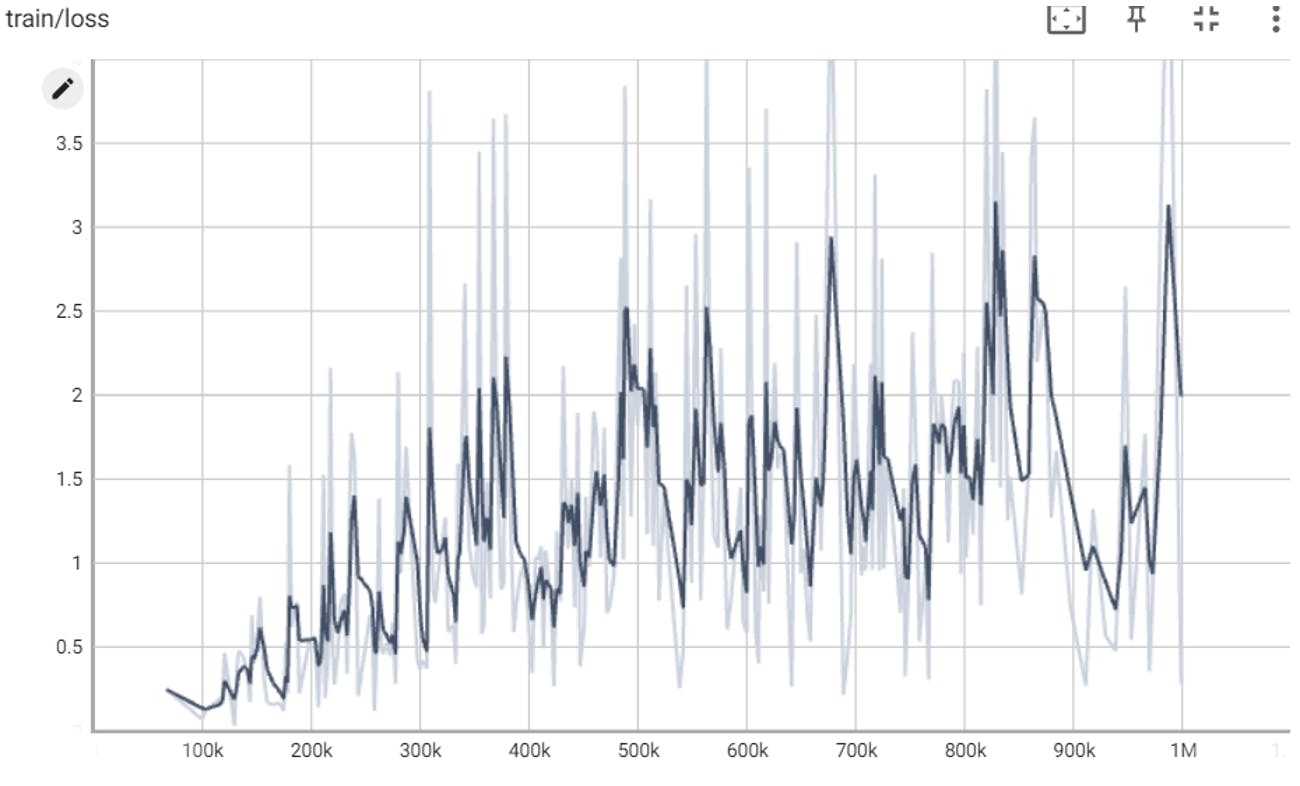
The loss parameter graph after 1,000,000 steps:

The loss parameter graph after 2,000,000 steps:

The loss parameter is a measure of how well the model is able to predict the Q-values of the state-action pairs. It is an indicator of how well the model is learning. If the loss is high, it means that the model is not able to predict the Q-values well, and if the loss is low, it means that the model is able to predict the Q-values well.
According to this graph, we can see the loss value goes up instead of down which points on a problem in the learning process, the model doesn’t predict the Q-Values well,
We think it arises from the change of the DQN Memory Buffer, it’s default (and recommended) size is 1,000,000 and we reduced it to 10,000 because of the available RAM size our computers have.
We think this change led to the fact that the stored experience DQN hold in the memory should be used fir learning purposes, so maybe decreasing its size caused some experience to not be in the memory for long enough for the model to learn from it, we severe the experience is deleted from the memory to fast for making room to newer experience.
But we can that the second graph is more stable than the first one, which can point on the fact that the model improved it’s ability to predict the Q-Values.
Real Time Comparison Between the Models
The comparison of both model will be done as follows:
We will compare each DQN model with its equivalent PPO model, equivalency will be based on the timesteps.
For simplicity, instead of comparing and analyzing every model we saved, we will compare only models that were saved after : 50,000 ; 500,000 ; 1,000,000 ; 2,000,000 timesteps.
We will conduct "regular" tests and 2 "special" tests.
Regular Tests:
Each "regular" test will include a link to a google drive folder that holds the videos of the 2 compared models running and playing the game.
The factors for comparison in each test will be:Most distance passed in the x-axis.
Dealing with obstacles (pipes, enemies, pits).
Highest score.
Rare staff findings (affected by the exploration rate).
Special Tests:
Each special tests will include a link to a google drive folder that holds the videos of the test.
The factors for comparison in each test will be:Can the model reach to level 2 of the game?
Testing each model on a new Mario environment the model never played or seen before (switching the environment from “Super Mario Bros1” to “Super Mario Bros2”) and testing according to regular test parameters.
Test 1
DQN vs PPO (50,000 timesteps models):videos
Most distance passed in the x-axis:
DQN:
Reached to the first green pipe.PPO:
Reached to the second green pipe.
Dealing with obstacles:
DQN:
Killed the first enemy mushroom and got stuck in the first green pipe.PPO:
Avoided the first enemy and Reached to the second green pipe.
Highest score:
DQN:
100 points.PPO:
0 points.
Rare staff findings:
- None found a rare item yet.
Conclusions:
Both algorithms are in the start of their learning process though we can see they managed to learn that jumping is good and that they need to jump in order to avoid some obstacles, PPO, in contrast to DQN learned how to jump higher and pass the first pipe, but DQN learned that he can jump on enemies, kill them and earn reward for that.
Test 2
DQN vs PPO (500,000 timesteps models):videos
Most distance passed in the x-axis:
DQN:
Reached to the first pit, couldn’t pass it.PPO:
Reached to the second pipe again, couldn’t pass it.
Dealing with obstacles:
DQN:
Deals with pipes better than in the first test, learned to jump high.Deals with enemies pretty good, jumps over them or kills them, but It’s still unstable, meaning sometimes he just run to them and die.
PPO:
Deals with pipes very weakly, still couldn’t pass the second pipe means it can’t jump high yet.Because it didn’t make it through the second pipe we can’t test dealing with enemies.
Highest score:
DQN:
200 points.PPO:
100 points.
Rare staff findings:
- None found a rare item yet.
Conclusions:
DQN is better than PPO on every aspect of the parameters and act the same when talking about finding rare items.
DQN is dealing with jumps and enemies better thus making it the better performing model.
Test 3
DQN vs PPO (1,000,000 timesteps models):videos
Most distance passed in the x-axis:
DQN:
Reached to the first pit, couldn’t pass it but in comparison to the last test tried to jump above the pit and failed .PPO:
Passed the first and second pits.
Dealing with obstacles:
DQN:
Ability to deal with pipes improved from the second test, learned to jump higher and smoother (See second 16 in video DQN_1M).Deals with enemies pretty good, jumps over them or kills them, but It’s still unstable, meaning sometimes he just run to them and die.
Tries to jump over the pit instead of just walking and falling to it, but still couldn’t pass it.
PPO:
Dealing with pipes is good but not stable.Dealing with enemies improved from the last test, kills and jumps over enemies.
Deals with pits pretty good when encounters them.
Highest score:
DQN:
400 points.PPO:
1000 points.
Rare staff findings:
DQN:
Couldn’t find any rare items.PPO:
Found 2 rare mushrooms that 1 of them was invisible, but didn’t take them
Conclusions:
DQN remained pretty stable with a little better adjustments, it leaned to coordinate jumps according to the agent’s velocity, which looks like almost a human made that jump and tried to jump over the second pit but still couldn’t pass it
On the other hand, PPO performance has spiked, in the previous test it couldn’t pass the second green pipe, and now it passed the DQN model performance in most parameter aspects, except that the DQN model jumps better.
Test 4
DQN vs PPO (2,000,000 timesteps models):videos
Most distance passed in the x-axis:
DQN:
Reached to the second pit and couldn’t pass it, managed to pass the first pit.PPO:
Passed the second pit and the turtle and couldn’t pass the 3 enemy mushrooms wave (See time 2:11 in video PPO_2M).
Dealing with obstacles:
DQN:
Dealing with pipes and enemies very smoothly.Succeeded to pass the first pit but couldn’t pass the second pit.
PPO:
Dealing with enemies and pipes is unstable, sometimes deals with them in a good way and sometimes doesn’t.Deals with the pits very good.
Overall performance is good but unstable.
Highest score:
DQN:
500 points.PPO:
500 points.
Rare staff findings:
- None found a rare item yet.
Conclusions:
The DQN model is stable, handles enemies and pipes very well, still has problems passing the pits, but overall, its performance is good.
The PPO model handles enemies and jumps in an unstable way, sometimes it does better than other times, deals with the pits very good and manages to pass the biggest distance (x-axis), so, overall had better performance than DQN.
Special Test 1
Question:
Can the model reach to level 2 of the game?
DQN:
The model never succeeded to pass the second pit.
PPO:
After 1 hour of model testing the model made it to level 2 (See the link to the video).
Conclusions:
PPO won the test.
Special Test 2
Testing each model on a new Mario environment the model has never played or seen before called Super Mario Bros 2.
Most distance passed in the x-axis:
DQN:
Passed the first long green pipe.PPO:
Passed the first long green pipe, passed the first pit failed at the second pit.
Dealing with obstacles:
DQN:
Dealing with pipes and enemies was pretty good, we could see that when the agent encounters a pipe, he knows that he should jump, but it had quite hard time dealing with the planes going out of the pipe that wasn’t exist in the training environment (Super Mario Bro 1).PPO:
Dealing with enemies and pipes was pretty good, did a good job on jumping near enemies and pipes and even jumped above the plants that go out from the pipes even though he is not familiar with them.The model knows that when it encounters a pit it should jump over it, so it managed learn that.
The overall performance of the model was very good.
Highest score:
DQN:
1700 points.PPO:
1600 points.
Rare staff findings:
DQN:
Found 1 rare mushroom (See second 0:46 In the video DQN_2M_SUPERMARIO2).PPO:
Found 1 rare mushroom and 1 rare star.
Conclusions:
PPO performance was better in the new environment, it manages to understand that he needs to jump above the plants, it manages to pass more distance on the x-axis, which is the main target reward function, so it made a better job in achieving the target.
Conclusions
Performance
Regarding the overall comparison, PPO performance is definitely better than DQN performance.
DQN is more stable in its performance, it handles pipes and enemies very well but failed miserably passing the pit.
On the other hand, PPO isn’t stable in it’s performance, most of the times it passes pipes and enemies and sometimes it can make stupid mistakes, but it reached level 2 of the game, and passed things in the game that the DQN model never reached to.
It even had better results while playing Super Mario Bros 2 (unfamiliar environment), thus it has better results overall and it achieved better convergence.
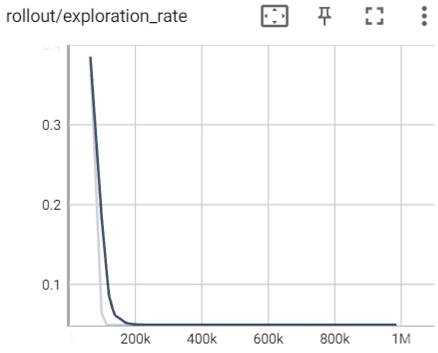
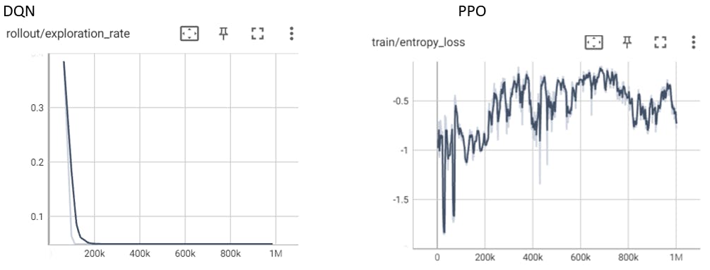
Exploration Rate
The tests prove that PPO found more rare things in the game, so we can assume it has a better exploration of the environment, that arises from the stochasticity of the policy to explore the environment.
PPO chooses the actions based on the states by a Bell distribution, meaning that even if it has found a good action for a certain state it will use it most of the times it encounters said state, but sometimes it will choose other actions with lower odds of occurrence for the purpose of exploration.
We can even see that in the graphs :
Personal Insights
We think that the PPO performance came on the strong hand because it is an on-policy algorithm that generates updates using the current policy as the agent explores the environment, which lead to a better and faster convergence, On the other hand the DQN is an off-policy algorithm that uses a memory buffer to store and reuse past experience so it’s learning is a bit slower.
One more important thing to add is that DQN memory buffer we used for training had relatively small size so we think a smaller buffer size may result in faster training but could also limit the ability of the algorithm to learn from long-term dependencies in the environment, which can explain the fact that DQN 500,000 timesteps model results were better than the PPO 500,000 timesteps model results (See regular test 2) but in the end PPO has converged to a better model and achieved better results.
The last conclusion is that more research needs to be done in order to determine solid facts, both models should be trained a lot more and achieve more stability.
References
The Environment
The Algorithms
Articles About The Algorithms
PPO
- Schulman, J., Wolski, F., Dhariwal, P., Radford, A., & Klimov, O. (2017). Proximal Policy Optimization Algorithms. CoRR, abs/1707.06347. https://arxiv.org/abs/1707.06347
DQN
Mnih, V., Kavukcuoglu, K., Silver, D., Graves, A., Antonoglou, I., Wierstra, D., & Riedmiller, M. (2013). Playing Atari with Deep Reinforcement Learning.
https://arxiv.org/pdf/1312.5602Mnih, V., Kavukcuoglu, K., Silver, D., et al. (2015). Human-level control through deep reinforcement learning. Nature, 518, 529–533. https://doi.org/10.1038/nature14236
Contributors
Lior Shilon.
Yair Davidof.
